
|
Figure 1: Hipparchus of Nicaea (c.190 – c.120 BC) at work Hipparchus, a Greek astronomer, invented the first scale to rate the brightness of the stars. |
When we look at the sky on a clear night we see stars. Some appear bright and others very faint as seen from Earth. Some of the faint stars are intrinsically very bright, but are very distant. Some of the brightest stars in the sky are very faint stars that just happen to lie very close to us. When observing, we are forced to stay on Earth or nearby and can only measure the intensity of the light that reaches us. Unfortunately this does not immediately tell us anything about a star’s internal properties. If we want to know more about a star, its size or physical/internal brightness, for example, we need to know its distance from Earth.
Historically, the stars visible to the naked eye were put into six different brightness classes, called magnitudes. This system was originally devised by the Greek astronomer Hipparchus about 120 BC and is still in use today in a slightly revised form. Hipparchus chose to categorise the brightest stars as magnitude 1, and the faintest as magnitude 6.
Astronomy has changed a lot since Hipparchus lived! Instead of using only the naked eye, light is now collected by large mirrors in either ground-based telescopes such as the VLT in the Atacama Desert in Chile or the Hubble Space Telescope above the Earth’s atmosphere. The collected light is then analysed by instruments able to detect objects billions of times fainter than any human eye can see.
However, even today astronomers still use a slightly revised form of Hipparchus’ magnitude scheme called apparent magnitudes. The modern definition of magnitudes was chosen so that the magnitude measurements already in use did not have to be changed. Astronomers use two different types of magnitudes: apparent magnitudes and absolute magnitudes.
The apparent magnitude, m, of a star is a measure
of how bright a star appears as observed on
or near Earth.
Instead of defining the apparent magnitude
from the number of light photons we observe,
it is defined relative to the magnitude and
intensity of a reference star. This means that an
astronomer can measure the magnitudes of stars
by comparing the measurements with some
standard stars that have already been measured
in an absolute (as opposed to relative) way.
The apparent magnitude, m, is given by:
m = mref – 2.5 log (I/Iref)
where mref is the apparent magnitude of the reference star, I is the measured intensity of the light from the star, and Iref is the intensity of the light from the reference star. The scale factor 2.5 brings the modern definition into line with the older, more subjective apparent magnitudes.
It is interesting to note that the scale that Hipparchus selected on an intuitive basis, using just the naked eye, is already logarithmic as a result of the way our eyes respond to light.
For comparison, the apparent magnitude of the full Moon is about –12.7, the magnitude of Venus can be as high as –4 and the Sun has a magnitude of about –26.5.
We now have a proper definition for the apparent magnitude. It is a useful tool for astronomers, but does not tell us anything about the intrinsic properties of a star. We need to establish a common property that we can use to compare different stars and use in statistical analysis. This property is the absolute magnitude.
The absolute magnitude, M, of a star is defined as the relative magnitude a star would have if it were placed 10 parsecs (read about parsecs in the Mathematical Toolkit if needed) from the Sun. Since only a very few stars are exactly 10 parsecs away, we can use an equation that will allow us to calculate the absolute magnitude for stars at different distances: the distance equation. The equation naturally also works the other way – given the absolute magnitude the distance can be calculated.
Figure 2: Temperature and colour of stars This schematic diagram shows the relationship between the colour of a star and its surface temperature. Intensity is plotted against wavelength for two hypothetical stars. The visible part of the spectrum is indicated. The star’s colour is determined by where in the visible part of the spectrum, the peak of the intensity curve lies. |
 |
 |
By the late 19th century, when astronomers
were using photographs to record the sky and to
measure the apparent magnitudes of stars, a
new problem arose. Some stars that appeared to
have the same brightness when observed with
the naked eye appeared to have different
brightnesses on film, and vice versa. Compared
to the eye, the photographic emulsions used
were more sensitive to blue light and less so to
red light.
Accordingly, two separate scales were devised:
visual magnitude, or mvis, describing how a star
looked to the eye and photographic magnitude,
or mphot, referring to measurements made with
blue-sensitive black-and-white film. These are
now abbreviated to mv and mp.
However, different types of photographic emulsions
differ in their sensitivity to different
colours. And people’s eyes differ too! Magnitude
systems designed for different wavelength
ranges had to be more firmly calibrated.
Today, precise magnitudes are specified by
measurements from a standard photoelectric
photometer through standard colour filters.
Several photometric systems have been devised;
the most familiar is called UBV after the three
filters most commonly used. The U filter lets
mostly near-ultraviolet light through, B mainly
blue light, and V corresponds fairly closely to
the old visual magnitude; its wide peak is in the
yellow-green band, where the eye is most sensitive.
The corresponding magnitudes in this system
are called mU, mB and mV.
Figure 3: Surface temperature versus B-V colour index This diagram shows the relation between the surface temperature of a star, T, and its B-V colour index. Knowing either the surface temperature or the B-V colour index you can find the other value from this diagram. |
 |
The term B-V colour index (nicknamed B-V by astronomers) is defined as the difference in the two magnitudes, mB-mV (as measured in the UBV system). A pure white star has a B-V colour index of about 0.2, our yellow Sun of 0.63, the orange-red Betelgeuse of 1.85 and the bluest star possible is believed to have a B-V colour index of –0.4. One way of thinking about colour index is that the bluer a star is, the more negative its B magnitude and therefore the lower the difference mB-mV will be. There is a clear relation between the surface temperature T of a star and its B-V colour index (see Reed, C., 1998, Journal of the Royal Society of Canada, 92, 36–37) so we can find the surface temperature of the star by using a diagram of T versus mB–mV(see Fig. 3).
log10(T) = (14.551 - (mB - mV) )/ 3.684
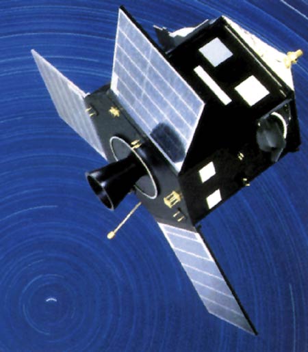 |
Figure 4: The ESA HIPPARCOS satellite The HIPPARCOS satellite was launched on the night of 8 August 1989 by a European Ariane 4 launcher. The principal objective of ESA's HIPPARCOS mission was the production of a star catalogue of unprecedented precision. The positions and the distances of a set of about 120,000 preselected stars with magnitudes down to B = 13 were determined with high accuracy. The HIPPARCOS mission ended in 1993 and the final star catalogue was published in 1997. |
The distance equation is written as:
m-M = 5 log (D/10 pc) = 5 log(D) – 5
This equation establishes the connection between the apparent magnitude, m, the absolute magnitude, M, and the distance, D, measured in parsec. The value m-M is known as the distance modulus and can be used to determine the distance to an object.
A little algebra will transform this equation to an equivalent form that is sometimes more convenient (feel free to test this yourselves):
D = 10(m-M+5)/5
When determining distances to objects in the Universe we measure the apparent magnitude m first. Then, if we also know the intrinsic brightness of an object (its absolute magnitude M), we can calculate its distance D. Much of the hardest work in finding astronomical distances is
concerned with determining the absolute magnitudes of certain types of astronomical objects. Absolute magnitudes have for instance been measured by ESA’s HIPPARCOS satellite. HIPPARCOS is a satellite that, among many other things, measured accurate distances and apparent magnitudes of a large number of nearby stars.
Up to now we have been talking about stellar magnitudes, but we have never mentioned how much light energy is really emitted by the star. The total energy emitted as light by the star each second is called its luminosity, L, and is measured in watts (W). It is equivalent to the power emitted.
Luminosity and magnitudes are related. A remote star with a high luminosity can have the same apparent magnitude as a nearby star with a low luminosity. Knowing the apparent magnitude and the distance of a star, we are able to The star radiates light in all directions so that its emission is spread over a sphere. To find the intensity, I, of light from a star at the Earth (the intensity is the emission per unit area), we divide its luminosity by the area of a sphere, with the star at the centre and radius equal to the distance of the star from Earth, D. See Fig. 5.
I = L/(4 pi D2)
The luminosity of a star can also be measured as a multiple of the Sun’s luminosity, Lsun = 3.85 × 1026 W. As the Sun is ‘our’ star and the best-known star, it is nearly always taken as the reference star.
Using some algebra we find the formula for calculating the luminosity, L, of a star relative to the Sun’s luminosity:
L/Lsun = (D/Dsun)2·I/Isun
The ratio I/Isun can be determined using the formula given in the Apparent Magnitudes section of the Astronomical Toolkit (msun = –26.5).
 |
Figure 5: Intensity of light This drawing shows how the same amount of radiation from a light source must illuminate an ever-increasing area as distance from the light source increases. The area increases as the square of the distance from the source, so the intensity decreases as the square of the distance increases. |